Mini project: plot an equity curve for a simple rule

This lesson puts the whole module to work in one script. You will take the moving-average signal from the previous lesson, turn it into an equity curve, compare it with simply buying and holding, measure the worst drawdown, and save a chart. Then you will do the step most beginners skip: check how much of the result is luck.

This is a first, simplified backtest. It ignores costs, assumes trades fill exactly at the close-to-close returns, and runs on synthetic data. Module 05 builds a more realistic one. The point here is to learn the mechanics, and to see early how little a single result can say.

The plan

The script does five things:

1. Generate two years of synthetic daily prices.
2. Compute daily returns and the 20/50 moving-average position, shifted one bar as before.
3. Build two equity curves from a starting capital of 10,000: one for the rule and one for buy and hold.
4. Summarise final equity, total return and maximum drawdown.
5. Plot both curves and save the chart to a file.

The script

Save this as equity_curve.py in your project and run it. It prints a summary and writes equity_curve.png to the same folder.

import matplotlib.pyplot as plt
import numpy as np
import pandas as pd
 
 
def make_prices(n_days=260, seed=42):
    """Synthetic daily OHLCV bars from a random walk. Not real market data."""
    rng = np.random.default_rng(seed)
    dates = pd.bdate_range("2024-01-01", periods=n_days, name="date")
    close = 100 * np.exp(np.cumsum(rng.normal(0.0003, 0.012, n_days)))
    prev_close = np.concatenate([[100.0], close[:-1]])
    open_ = prev_close * (1 + rng.normal(0, 0.002, n_days))
    high = np.maximum(open_, close) * (1 + np.abs(rng.normal(0, 0.004, n_days)))
    low = np.minimum(open_, close) * (1 - np.abs(rng.normal(0, 0.004, n_days)))
    volume = rng.integers(800_000, 1_500_000, n_days)
    return pd.DataFrame(
        {"open": open_, "high": high, "low": low, "close": close, "volume": volume},
        index=dates,
    )
 
 
def max_drawdown(equity):
    """Largest fall from a running peak, as a negative fraction."""
    return (equity / equity.cummax() - 1).min()
 
 
START_CAPITAL = 10_000
FAST, SLOW = 20, 50
 
prices = make_prices(n_days=500, seed=42)
df = pd.DataFrame({"close": prices["close"]})
df["ret"] = df["close"].pct_change().fillna(0)
 
fast_ma = df["close"].rolling(FAST).mean()
slow_ma = df["close"].rolling(SLOW).mean()
df["signal"] = (fast_ma > slow_ma).astype(int)
df["position"] = df["signal"].shift(1).fillna(0)
 
df["rule_equity"] = START_CAPITAL * (1 + df["position"] * df["ret"]).cumprod()
df["hold_equity"] = START_CAPITAL * (1 + df["ret"]).cumprod()
 
rule_final = df["rule_equity"].iloc[-1]
hold_final = df["hold_equity"].iloc[-1]
summary = pd.DataFrame(
    {
        "final equity": [rule_final, hold_final],
        "total return %": [100 * (rule_final / START_CAPITAL - 1), 100 * (hold_final / START_CAPITAL - 1)],
        "max drawdown %": [100 * max_drawdown(df["rule_equity"]), 100 * max_drawdown(df["hold_equity"])],
    },
    index=[f"MA {FAST}/{SLOW} rule", "Buy and hold"],
)
print(summary.round(1))
print("Entries:", int((df["position"].diff() == 1).sum()))
print(f"Time in the market: {df['position'].mean():.0%}")
 
plt.style.use("dark_background")
fig, ax = plt.subplots(figsize=(10, 5))
ax.plot(df.index, df["rule_equity"], color="white", linewidth=1.6, label=f"MA {FAST}/{SLOW} rule")
ax.plot(df.index, df["hold_equity"], color="gray", linewidth=1.2, label="Buy and hold")
ax.axhline(START_CAPITAL, color="dimgray", linewidth=0.8, linestyle="--")
ax.set_title("Equity curves on synthetic data (educational example)")
ax.set_ylabel("Equity ($)")
ax.legend(loc="upper left")
fig.tight_layout()
fig.savefig("equity_curve.png", dpi=150)

               final equity  total return %  max drawdown %
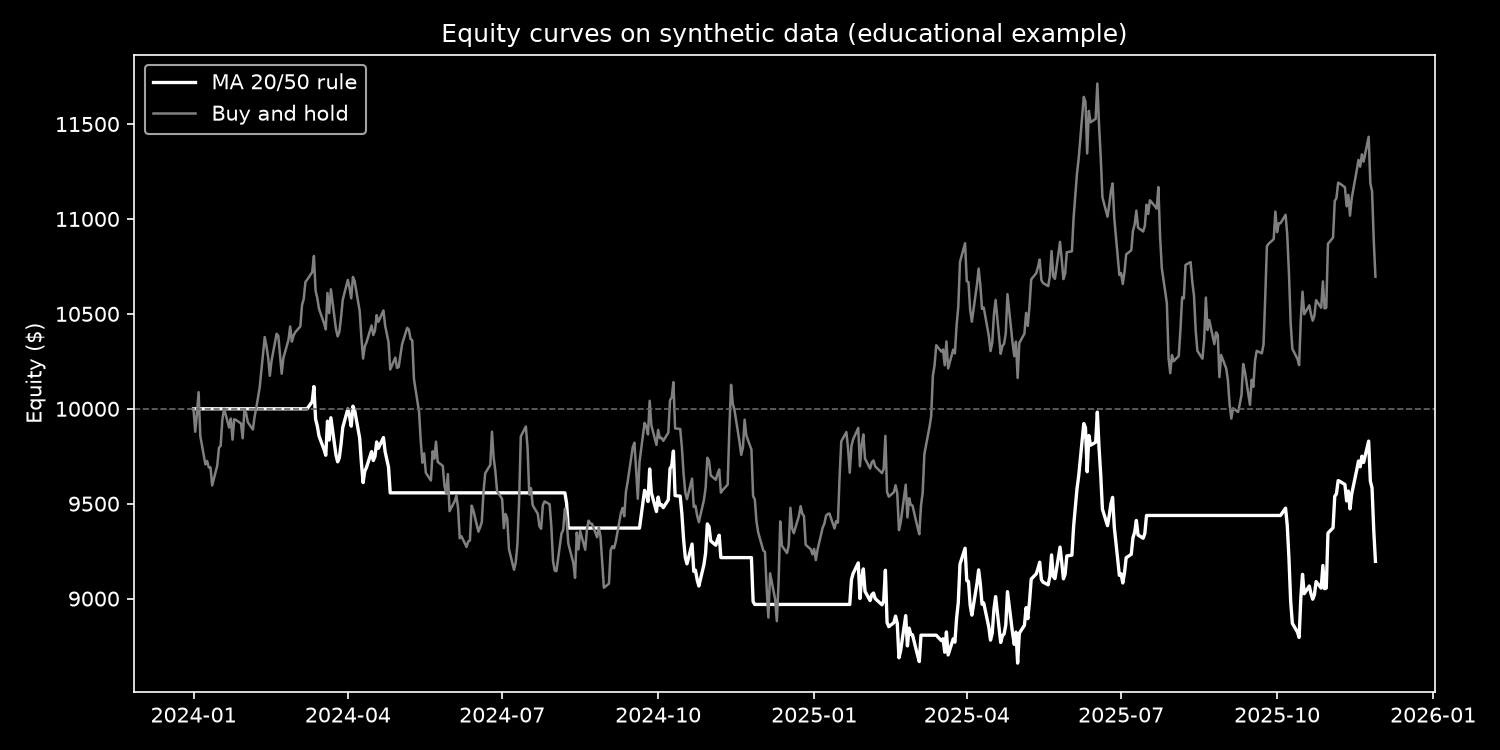
MA 20/50 rule        9196.2            -8.0           -14.4
Buy and hold        10696.0             7.0           -17.8
Entries: 7
Time in the market: 46%

How it works

Settings in capitals. START_CAPITAL, FAST and SLOW are written in capital letters, a Python convention for values that are set once and not changed. Keeping them at the top means you can try a different rule by editing one line, and the chart labels update themselves through the f-strings. The line FAST, SLOW = 20, 50 assigns two variables at once.

The equity curves. The highlighted lines are the heart of the script. df["position"] * df["ret"] is the strategy's daily return: the market's return on days the rule is long, zero on days it is flat. Adding 1 turns each return into a growth factor, so a 1% gain becomes 1.01. .cumprod() multiplies the factors cumulatively, day by day, which is compounding, and multiplying by the starting capital turns that into money. The equity curve for buy and hold is the same calculation with the position always 1.

Drawdown. equity.cummax() is the highest equity reached so far on each day. Dividing the equity by that running peak and subtracting 1 gives the drawdown: how far below its best level the account is, as a negative fraction. The minimum of that series is the maximum drawdown, the worst peak-to-trough fall in the test.

The summary table. A DataFrame does not have to hold dated rows. Here it holds two rows, one per approach, with readable labels as the index. The list after each column name gives the rule's value and then buy and hold's.

Counting entries. .diff() == 1 is True on days the position went from 0 to 1. Summing booleans counts the True values, because True counts as 1.

The chart. matplotlib.pyplot, imported as plt, is Python's standard plotting library. plt.subplots() creates a figure (the image) and axes (the plotting area inside it). Each ax.plot(...) draws one line, ax.axhline draws the starting capital as a dashed reference, and ax.legend labels the lines. fig.savefig writes the file. The dark_background style is optional; delete that line for matplotlib's default look. In JupyterLab, the chart also appears below the cell; in a script, open the saved file, or add plt.show() at the end to open a window.

Here is the chart the script produces:

Reading the result

On this price path, the rule lost 8% while buy and hold made 7%. The rule's worst drawdown was smaller, 14.4% against 17.8%, mostly because it spent more than half the time out of the market; the flat stretches in the chart are the periods it was in cash.

It would be easy to tell a story about this: the rule protects capital but lags in rising markets. Before telling any story, ask how much of the result is luck. With synthetic data, you can answer that directly by changing the seed and running the same rule on different random paths.

import numpy as np
import pandas as pd
 
 
def make_prices(n_days=260, seed=42):
    """Synthetic daily OHLCV bars from a random walk. Not real market data."""
    rng = np.random.default_rng(seed)
    dates = pd.bdate_range("2024-01-01", periods=n_days, name="date")
    close = 100 * np.exp(np.cumsum(rng.normal(0.0003, 0.012, n_days)))
    prev_close = np.concatenate([[100.0], close[:-1]])
    open_ = prev_close * (1 + rng.normal(0, 0.002, n_days))
    high = np.maximum(open_, close) * (1 + np.abs(rng.normal(0, 0.004, n_days)))
    low = np.minimum(open_, close) * (1 - np.abs(rng.normal(0, 0.004, n_days)))
    volume = rng.integers(800_000, 1_500_000, n_days)
    return pd.DataFrame(
        {"open": open_, "high": high, "low": low, "close": close, "volume": volume},
        index=dates,
    )
 
 
def ma_rule_vs_hold(prices, fast=20, slow=50):
    """Total return of the moving-average rule and of buy and hold, as fractions."""
    close = prices["close"]
    ret = close.pct_change().fillna(0)
    signal = (close.rolling(fast).mean() > close.rolling(slow).mean()).astype(int)
    position = signal.shift(1).fillna(0)
    rule = (1 + position * ret).prod() - 1
    hold = (1 + ret).prod() - 1
    return rule, hold
 
 
for seed in range(1, 6):
    rule, hold = ma_rule_vs_hold(make_prices(n_days=500, seed=seed))
    print(f"Seed {seed}: MA rule {rule:+6.1%}   buy and hold {hold:+6.1%}")

Seed 1: MA rule  -4.9%   buy and hold  -6.7%
Seed 2: MA rule -24.4%   buy and hold -15.9%
Seed 3: MA rule +24.0%   buy and hold +57.6%
Seed 4: MA rule +23.8%   buy and hold +19.7%
Seed 5: MA rule +18.4%   buy and hold +18.2%

The function returns two values at once, separated by a comma, and rule, hold = ... unpacks them into two variables. In the format code, +6.1% shows a sign, one decimal and a width of six characters, so the columns line up.

Same rule, same settings, five random paths: the results run from −24.4% to +24.0%. The rule beats buy and hold on some paths and trails it on others. None of this says anything about the rule, because a random walk contains no trends for a trend rule to find. It says a great deal about single backtests: one equity curve is one draw from a wide range of possible outcomes.

What this module gave you

You can now set up a Python project, write functions, hold price data in pandas, compute returns and indicators, time a signal correctly, and turn it into an equity curve with a benchmark and a drawdown. That is enough to start asking real questions. The next module looks at the data those questions depend on, and the ways it can mislead you before a single line of strategy code runs.